Practical Examination: Impact of Learning Rate on ML and DL Model's Performance

I am a self-taught Python developer who loves to write on Python Programming and quite obsessed with Machine Learning.
In this tutorial, you'll look at how learning rate affects ML (Linear Regression Model) and DL (Neural Networks) models, as well as which adaptive learning rate methods best optimize neural networks in deep learning.
What is the Learning Rate?
Learning rate is a hyperparameter that tunes the step size of the model's weights during each iteration of the optimization process. The learning rate is used in optimization algorithms like SGD (Stochastic Gradient Descent) to minimize the loss function that enhances the model's performance.
The step size, determined by the learning rate, decides how much the model's weights are updated in each iteration towards the gradient of the loss function. The learning rate can be dynamically adjusted during training to help the model reach the best possible performance.
Impact of Learning Rate on Model's Performance
A higher learning rate causes the model's weights to take larger steps on each iteration towards the gradient of the loss function. While this can lead to faster convergence, it can also result in instability and poorer performance.
In the case of a lower learning rate, the model's weights are updated by small steps causing slower convergence towards the optimal performance. Although it takes more time to train, it often offers greater stability and a better chance of reaching an optimal performance.
Practical Example
This section will cover the practical examples of using learning rate to understand its impact on the machine and deep learning models. Additionally, you'll see how adaptive learning rate methods help in optimizing the deep learning model's performance.
Impact of Learning Rate on Machine Learning Model
In this section, you'll use the SGDRegressor model provided by Scikit Learn that provides leverage to use the learning rate parameter.
Grab the dataset from here.
Importing Required Modules
import pandas as pd
import matplotlib.pyplot as plt
from sklearn.model_selection import train_test_split
from sklearn.linear_model import SGDRegressor
from sklearn.metrics import mean_squared_error
The pandas library will be used for reading the dataset whereas matplotlib.pyplot will be used for plotting the learning curves.
The train_test_split function from the Scikit-Learn library will be employed to split the dataset into training and testing batches. Additionally, the mean_squared_error function from Scikit-Learn's metrics module will be used to calculate the differences between the actual and predicted values.
The SGDRegressor class will be used for fitting the linear regression model that uses stochastic gradient descent (SGD) for optimization.
Loading the Data
# Load the data
df = pd.read_csv("D:/SACHIN/Jupyter/LRImpact/bmi_data.csv")
# Separating Feature and Target Variables
X = df[['Height', 'Weight', 'Gender']]
y = df['Index']
The data is read from the specified CSV file using the pd.read_csv() function, and the resulting DataFrame is stored inside the df variable.
The features of the dataset are separated and stored inside the X variable. Similarly, the target variable, denoted as "Index", is separated from the dataset and stored inside the y variable.
Preparing Data for Training
# Preparing Data for training
X_train, X_test, y_train, y_test = train_test_split(X, y, test_size=0.3, random_state=42)

# List of Learning rates
learning_rates = [0.0001, 0.001, 0.01, 0.1, 0.2, 0.5, 0.8, 1]
# Empty List for storing errors
train_errors_list = []  # To store train errors
test_errors_list = []  # To store test errors
The data is split into training and testing sets, specifically into X_train, X_test, y_train, and y_test using the train_test_split() function, where both features (X) and the target (y) are provided as input. The test_size parameter is set to 30% of the dataset, and the random_state is set to 42 for reproducibility.
A list of learning rates is defined, the model will run for each value in the learning_rates list, and two empty lists are created named train_errors_list (store training errors) and test_errors_list (store test errors).
Training Model with SGDRegressor
for i in range(len(learning_rates)):
    model = SGDRegressor(learning_rate='constant', eta0=learning_rates[i], random_state=42)

    train_errors = []
    test_errors = []

    for _ in range(200):
        model.partial_fit(X_train, y_train)

        y_train_pred = model.predict(X_train)
        y_test_pred = model.predict(X_test)

        train_error = mean_squared_error(y_train, y_train_pred)
        test_error = mean_squared_error(y_test, y_test_pred)

        train_errors.append(train_error)
        test_errors.append(test_error)

    train_errors_list.append(train_errors)
    test_errors_list.append(test_errors)
A loop is initiated to iterate over the list of learning rates. This loop will run for the same number of iterations as there are learning rates in the list.
Inside the loop, the SGDRegressor model is instantiated with specific parameters: learning_rate is set to 'constant' (which is the default setting), and eta0 is set to learning_rates[i], signifying that the learning rate varies for each iteration.
Two empty lists, train_errors and test_errors, are created to collect the training and testing errors, respectively.
Within the loop, another loop is created to run the model for 200 epochs or iterations.
During each epoch, the model is updated with training data in small batches using the partial_fit method, which represents incremental learning.
Following the update, the model's predictions for both the training and testing data are stored in y_train_pred and y_test_pred, respectively.
The mean squared error is then computed between the actual target values (y_train and y_test) and the predicted target values (y_train_pred and y_test_pred) to evaluate how well the model fits the data.
The training and testing errors for each epoch are stored in the train_errors and test_errors lists, respectively.
Upon completing 200 epochs for each learning rate, the accumulated training and testing errors are appended to the train_errors_list and test_errors_list, respectively.
Plotting Learning Curves
# Plot learning curves for each learning rate
for i in range(len(learning_rates)):
    plt.subplot(4, 2, (i + 1))
    plt.plot(train_errors_list[i], label='train')
    plt.plot(test_errors_list[i], label='test')
    plt.legend()
    plt.suptitle('Impact of Learning Rates on Linear Regression')
    plt.title('LR = ' + str(learning_rates[i]))

plt.show()
To plot the learning curves for each learning rate, a loop is created to iterate over the length of learning rates from the list learning_rates.
Within the loop, the grid of subplots is created with 4 rows and 2 columns using plt.subplot(4, 2, (i + 1), and i+1 is used to specify the index number of the subplot.
Two lines are plotted within each subplot: train_errors_list[i] (training errors for a specific learning rate) and test_errors_list[i] (testing errors for a specific learning rate).
Each subplot's legend and title are customized, and the supertitle is customized for the entire grid of subplots.
Finally, the plt.show() function is used to display the entire grid of subplots.
Result
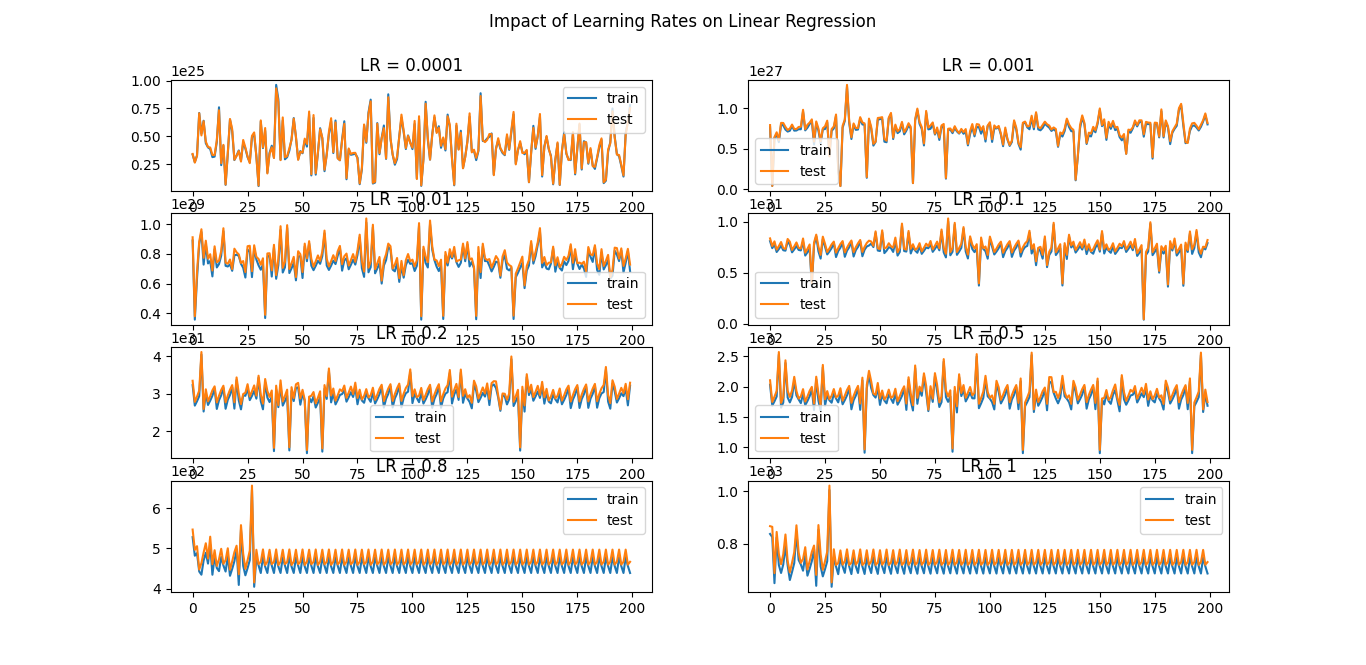
The model with learning rates of 0.001 and 0.01 performed well, but the model with a learning rate of 0.1 performed significantly better. Despite the slower convergence, the stability is excellent.
You can experiment with various values, such as changing the learning rates and increasing or decreasing the number of epochs.
Note: Your results may vary, you can try running the model 2-3 times for the average outcome.
Impact of Learning Rate on Deep Learning Model
In this section, you will examine the effect of learning rates on neural networks using Keras' SGD optimizer, as well as the effect of momentum on performance by accelerating the training process. Then you'll see which optimizer optimizes the neural networks the best.
Importing Required Modules
import pandas as pd
import matplotlib.pyplot as plt
from tensorflow.keras.models import Sequential
from tensorflow.keras.layers import Dense
from tensorflow.keras.optimizers import SGD
from tensorflow.keras.utils import to_categorical
The Sequential class will be used to stack neural network layers, the Dense layer will be used to add fully connected layers to the neural network architecture, the SGD optimizer will be essential for applying learning rate and momentum to the neural network, and to_categorical will be used for one-hot encoding.
Loading the Data
# Reading data
df = pd.read_csv("D:/SACHIN/Jupyter/LRImpact/bmi_data.csv")
X = df[['Height', 'Weight', 'Gender']]
y = df['Index']
The data is read and the resulting DataFrame is stored inside the df variable.
The features of the dataset are separated and stored inside the X variable. Similarly, the target variable, denoted as "Index", is separated from the dataset and stored inside the y variable.
Preparing the Data
# One-hot Encoding the Target Variable
y = to_categorical(y)

# Preparing Data for Training
param = 300
X_train, X_test = X[:param], X[param:]
y_train, y_test = y[:param], y[param:]
First, The target variable y undergoes one-hot encoding using the to_categorical() function to convert it into a 2D array of binary vectors suitable for multi-class classification problems.
The dataset is divided into two batches: training and testing. The split point is determined by the param variable.
The X_train variable contains samples from start (index=0) to 299 (index=299) and the X_test variable holds samples from 300 up to the end. The same is done with the y_train and y_test variables.
# Empty list for storing the training data accuracy
acc = []
# Empty list for storing the validation data accuracy
val_acc = []

# List of learning rates
learning_rates = [1, 0.1, 0.01, 0.001, 0.0001, 0.00001, 0.000001, 0.0000001]
Two empty lists are created: acc will collect accuracy values from the training data and val_acc will store accuracy values from the validation data.
The learning_rates variable defines a list of various learning rates.
Training the Neural Networks
for i in range(len(learning_rates)):
    model = Sequential()

    model.add(Dense(128, input_shape=(3, ), activation='relu'))
    model.add(Dense(64, activation='relu'))
    model.add(Dense(6, activation='softmax'))

    optimize = SGD(learning_rate=learning_rates[i])

    model.compile(optimizer=optimize, loss='categorical_crossentropy', metrics=['accuracy'])

    result = model.fit(X_train, y_train, validation_data=(X_test, y_test), epochs=200, verbose=0)

    acc.append(result.history['accuracy'])
    val_acc.append(result.history['val_accuracy'])
The loop iterates over the learning rates, and for each learning rate, a neural network model is created and trained.
Inside the loop, the instance of the Sequential is created and stored inside the model variable.
Following that, the neural network has one input layer and one hidden layer with 128 and 64 nodes, respectively, using the ReLU activation function. The output layer has 6 nodes (output classes) and uses the softmax activation function.
The instance of SGD optimizer is created in which the learning_rate parameter is set to learning_rates[i] which means the learning rate changes for each iteration, allowing you to test different learning rates.
The model is compiled with the specified optimizer (optimize), loss function (categorical_crossentropy for multi-class classification), and the metric to be monitored during training (accuracy).
The model is trained using X_train and y_train for 200 epochs (epochs=200) and validated on X_test and y_test. The training results are stored in the result variable.
The accuracy values for both training and validation data are collected for each learning rate. Training accuracy is stored in the acc list, and validation accuracy is stored in the val_acc list using result.history['accuracy'] and result.history['val_accuracy'].
Plotting
# Plot learning curves for each learning rate
for i in range(len(learning_rates)):
    plt.subplot(4, 2, (i + 1))
    plt.plot(acc[i], label='train')
    plt.plot(val_acc[i], label='test')
    plt.legend()
    plt.title('LR = ' + str(learning_rates[i]))
    plt.suptitle("Impact of LR on Multi-class Classification Model")

plt.show()
For each learning rate, a grid of subplots (4 rows and 2 columns) is created and within each subplot, two lines will be plotted acc[i] (training data accuracy for a specific learning rate) and val_acc[i] (validation data accuracy for a specific learning rate).
Finally, the entire grid of subplots is displayed using the plt.show() function.
Result

You can see that the model did well for the learning rates of 0.001, 0.0001, and 0.00001. The convergence is slow and takes more training time but the model has shown great stability and performance.
Note: Your results may vary, you can try running the model 2-3 times for the average outcome.
Using Momentum
The SGD optimizer offers a momentum parameter that, when utilized, can help accelerate the training process by allowing the optimizer to build up velocity and smoothen the progression during optimization.
import pandas as pd
import matplotlib.pyplot as plt
from tensorflow.keras.models import Sequential
from tensorflow.keras.layers import Dense
from tensorflow.keras.optimizers import SGD
from tensorflow.keras.utils import to_categorical

# Reading data
df = pd.read_csv("D:/SACHIN/Jupyter/LRImpact/bmi_data.csv")
X = df[['Height', 'Weight', 'Gender']]
y = df['Index']

# One-hot Encoding the Target Variable
y = to_categorical(y)

# Preparing Data for Training
param = 300
X_train, X_test = X[:param], X[param:]
y_train, y_test = y[:param], y[param:]

# Empty list for storing the training data accuracy
acc = []
# Empty list for storing the validation data accuracy
val_acc = []

# List of Momentum
mom = [0.0, 0.1, 0.5, 0.9]

for i in range(len(mom)):
    model = Sequential()

    model.add(Dense(128, input_shape=(3,), activation='relu'))
    model.add(Dense(64, activation='relu'))
    model.add(Dense(6, activation='softmax'))

    optimize = SGD(learning_rate=0.001, momentum=mom[i])

    model.compile(optimizer=optimize, loss='categorical_crossentropy', metrics=['accuracy'])

    result = model.fit(X_train, y_train, validation_data=(X_test, y_test), epochs=200, verbose=0)

    acc.append(result.history['accuracy'])
    val_acc.append(result.history['val_accuracy'])

# Plot learning curves for each momentum value
for i in range(len(mom)):
    plt.subplot(2, 2, (i + 1))
    plt.plot(acc[i], label='train')
    plt.plot(val_acc[i], label='test')
    plt.legend()
    plt.title('Momentum = ' + str(mom[i]))
    plt.suptitle("Impact of Momentum")

plt.show()
In the above code, a learning rate of 0.001 is taken. This learning rate has shown reasonable performance in previous experiments when training neural networks.
Different values of momentum are stored in the mom list. The code iteratively applies these momentum values to the model.
The highlighted line of code initializes an instance of the SGD optimizer. It configures the optimizer with a fixed learning rate of 0.001 and a momentum value specified by mom[i]. This means that for each iteration, the momentum value changes according to the elements of the mom list.
The code creates a grid of subplots with 2 rows and 2 columns to visualize the learning curves for different momentum values.
Finally, learning curves are plotted for each momentum value, showing both training and validation accuracy over epochs.
Result
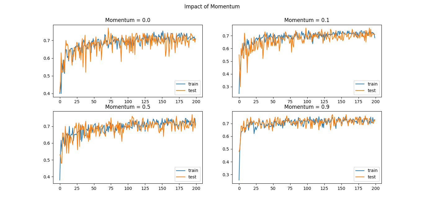
You can see that the momentum accelerated the training process of the model and a momentum value of 0.9 achieved approximately maximum train and test accuracy within 70 or fewer epochs and after that, the learning curve stayed almost constant.
Various Optimizers for Model Optimization
In this section, you will see how various optimizers impact the training process of the model with their default setting.
Keras provides a variety of optimizers that uses stochastic gradient descent algorithm with adaptive learning rates. The following optimizers will be used for optimizing the model's training process.
Code
import pandas as pd
import matplotlib.pyplot as plt
from tensorflow.keras.models import Sequential
from tensorflow.keras.layers import Dense
from tensorflow.keras.utils import to_categorical

# Reading data
df = pd.read_csv("D:/SACHIN/Jupyter/LRImpact/bmi_data.csv")
X = df[['Height', 'Weight', 'Gender']]
y = df['Index']

# One-hot Encoding the Target Variable
y = to_categorical(y)

# Preparing Data for Training
param = 300
X_train, X_test = X[:param], X[param:]
y_train, y_test = y[:param], y[param:]

# Empty list for storing the training data accuracy
acc = []
# Empty list for storing the validation data accuracy
val_acc = []

# List of Optimizers
optimizers = ['adamax', 'adam', 'adagrad', 'rmsprop']

for i in range(len(optimizers)):
    model = Sequential()

    model.add(Dense(128, input_shape=(3,), activation='relu'))
    model.add(Dense(64, activation='relu'))
    model.add(Dense(6, activation='softmax'))

    optimize = optimizers[i]

    model.compile(optimizer=optimize, loss='categorical_crossentropy', metrics=['accuracy'])

    result = model.fit(X_train, y_train, validation_data=(X_test, y_test), epochs=200, verbose=0)

    acc.append(result.history['accuracy'])
    val_acc.append(result.history['val_accuracy'])

# Plot learning curves for different optimizers
for i in range(len(optimizers)):
    plt.subplot(2, 2, (i + 1))
    plt.plot(acc[i], label='train')
    plt.plot(val_acc[i], label='test')
    plt.legend()
    plt.title('Optimizer = ' + str(optimizers[i]))
    plt.suptitle("Impact of Optimizer")

plt.show()
Result
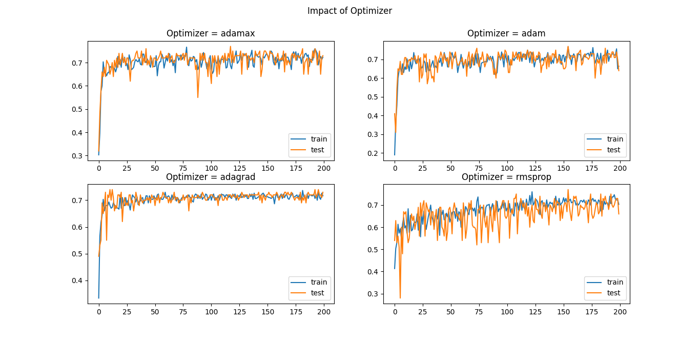
The 'adamax' and 'adam' exhibit nearly identical performance when converging towards the optimal state, 'adagrad' learned the problem within 60 epochs and then did not converge further. In the case of 'rmsprop', you can see excessive fluctuations in testing accuracy compared to training accuracy while converging, it learned the problem but requires more epochs.
Conclusion
In this tutorial, you've learned how different learning rates affect machine learning and neural network models. You first explored this with Scikit-learn's SGDRegressor model and then with Keras's SGD optimizer for a multi-class classification problem. Additionally, you saw how momentum can speed up training.
In the final part, you tested various optimizers such as Adamax, Adam, Adagrad, and RMSprop with neural networks to find out which one works best.
🏆Other articles you might be interested in if you liked this one
✅How to build a custom deep learning model using the transfer learning technique?
✅How to build a Flask image recognition app using a deep learning model?
✅What are Sessions and how to use them in a Flask app as temporary storage?
✅How to structure a flask app using Flask Blueprint?
✅Upload and display images on the frontend using Flask in Python.
✅How to connect the SQLite database with the Flask app using Python?
That's all for now
Keep Coding✌✌


